一篇文檔翻譯,內有m文件,現在貢獻出來,希望對你們有幫助
經典最大熵(ME)的問題包括根據已知函數的有限期望集確定概率分布函數(pdf)。該解決方案取決于$ N + 1 $拉格朗日乘數,該乘數是通過求解由$ N $數據約束和歸一化約束形成的非線性方程組確定的。在這段簡短的論文中,我們給出了三個Matlab程序來計算這些拉格朗日乘數。第一個考慮了功能可以是任何功能的一般情況。第二個考慮冪函數$ x ^ n $的特殊情況。在這種情況下,數據是$ p(x)$的幾何矩。第三部分考慮傅立葉級數函數$ \ exp(-jn \ omega x)$的特殊情況。在這種情況下,數據為$ p(x)$的三角矩。
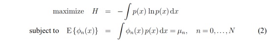
Shannon (1948)指出最大熵(ME)分布是如何通過變分法的直接應用而得到的。他定義概率密度函數p(x)的熵為
在文獻中,已知求H的最大值是一種方法,它可以得到最小信息先驗分布的形式;Jaynes(1968)和Zellner(1977)。Jaynes(1982)廣泛地分析了離散情況下的例子,而在Lisman and Van Znylen(1972)、Rao(1973)和Gokhale(1975)中,考慮了Kagan、Linjik連續情況。在最后一種情況下,問題的一般形式如下
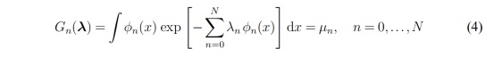
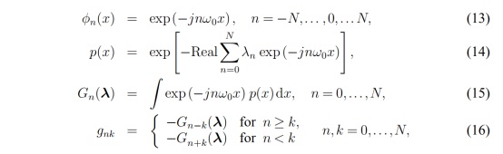
μ0 = 1,φ0 (x) = 1,φn (x), n = 0,……N, N是已知函數,μn N = 0,……,N是給定的期望數據。給出了該問題的經典解
(N + 1) Lagrangien參數λ=[λ0,……,λn] 通過 解決 following 組 (N + 1 ) 非線性方程
3式定義的分布形式大量已知的分布,通過選擇適當的N和φn areobtained (x), N = 0,…, N。一般φn (x) areeither x或者x的對數的權力。看到Mukhrejee和赫斯特(1984),Zellner (1988), Mohammad-Djafari(1990)對許多其他的例子和討論。許多作者廣泛地分析和使用了一些特殊的案例。當φn (x) = xn, n = 0,……Nμn, N = 0,……,N是給定的N個分布矩。參見Zellner(1988)在N = 4的情況下的數值實現。
在這個部分我們提出三個用MATLAB編寫的程序來解決方程組(4)。首先是一個通用的程序,φn (x)可以是任何功能。第二個是一個特殊情況φn (x) = xn, n = 0,…, n。在這種情況下,μn幾何p (x)的時刻。第三個是特殊情況φn (x) = exp (?jnωx), n = 0,…, n。在這種情況下,μn的三角時刻(Fouriercomponents) p (x)。我們也給出了一些例子來說明這些程序的用處。 函數原理我們已經看到標準的解決我的問題是由(3)的拉格朗日乘數法λ是通過求解非線性方程(4)。一般情況下,這些方程都是用標準牛頓法求解的,該方法是將泰勒級數中的Gn(λ)展開到lambda的試值附近,去掉二次項和高階項,迭代求解得到的線性系統。我們在這里給出了我們實現的數值方法的細節。當在試驗λ0附近展開一階泰勒級數的方程(4)中的Gn(λ)時,得到的線性方程由
注意向量δ和v 矩陣G 則式(5)變為
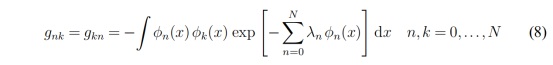
這個系統是求解δ的,我們從δ中驅動λ=λ0+δ,這將成為我們的新初始向量λ0,迭代將繼續,直到δ變得適當小。注意矩陣G是對稱的,我們有
因此,在每次迭代中,我們都要計算式(8)中的N(N?1)/2的積分,一般最大熵問題的算法如下: - 計算式(4)中的(N + 1)積分和矩陣G的N(N?1)/2個不同元素gnk,通過計算式(8)
- 解方程(7)找到δ
 - 計算λ=λ0 +δ,回到第三步,直到δ變得很小
方程(4)和(8)的積分可以用單變量森普森方法進行計算。 我們使用了這個方法的一個非常簡單的版本
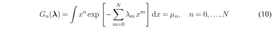
幾何矩的情況現在考慮時間問題的特殊情況,φn (x) = xn, n = 0,…, n。
在這種情況下,方程(3)(4)(8) beco
這意味著 [(N +1)×(N +1)] 在方程矩陣 G (7) 成為 symmetric Hankel 矩陣完全由 2 N Gn(λ),n = 0 ,...,2N. + 1 的值因此,本例中的算法與前面的算法相同,只是做了兩個簡化。
- 在步驟2中我們不需要編寫一個獨立函數計算functionsφn (x) = xn, n = 0,…
- 在步驟4積分估值的減少,是因為元素gnkof矩陣G相關積分Gn(λ)方程(10)。這個矩陣完全由2N + 1個分量定義.
三角函數的例子另一個有趣的特殊情況是數據是p(x)的傅里葉部分
μn可能是復數的和存在值μ(下標?n)=μn。這意味著他們有以下關系 因此矩陣G的所有元素都與p(x)的離散傅里葉變換有關。注意,G是厄米特的托普利茲矩陣
實例和數值實驗為了說明所提出的程序的有用性,我們首先考慮伽瑪分布的情況
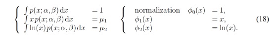
當約束條件為下列式子時,該分布可視為ME分布
因此很容易得到,方程(12)可以寫成 現在考慮以下問題 鑒于μ1和μ2確定λ0,λ1和λ
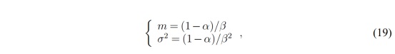
這可以通過標準ME方法來完成。要做到這一點,首先我們必須定義rangeof x (xmin xmax, dx),和寫一個函數fi_x計算functionsφ0 (x) = 1,φ1 (x) = x和φ2 (x) = lnx(參見附件中的函數fin1_x)。然后我們必須定義一個初始估計λ0λ,最后,讓程序工作。 分析(α,β)和m = E {x}和均值方差σ2 = E {(x?m) 2}之間的關系你會發現他們,伽馬分布的情況很有意思 或者反過來 這樣我們就可以利用這些關系來確定m和σ。也要注意類似的熵的最終結果是函數的副產品表(1)給出了ME_DENS1程序得到的一些統計結果(見附件)
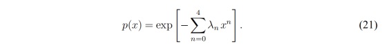
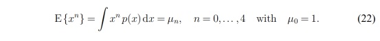
下一個例子是四次分布 當約束條件為此時,該分布可以認為是一個ME分布
現在考慮以下問題:給定的n,n = 1,…4計算出n,n = 0,…4。這可以由ME_DENS2程序完成。表(2)通過這個程序給出了一些數值結果 這些例子展示了如何使用建議的程序。第三個例子是在附件中,它展示了如何使用ME_DENS3程序來考慮三角矩的情況
總結本文中,我們先解決我的類分布當可用數據afinite組期望μn = E{φn (x)}一些已知函數φn (x), n = 0,…, n。我們提出三個Newton-Raphsonmethod Matlab程序來解決這一問題的一般情況下,對于幾何數據,時刻φn (x) = xn和三角的時刻φn (x) = exp (?jnω0x)。最后,給出了一些具體算例的數值結果
附頁
1 function [lambda,p,entr]=me_dens1(mu,x,lambda0)
2 %ME_DENS1
3 % [LAMBDA,P,ENTR]=ME_DENS1(MU,X,LAMBDA0)
4 % This program calculates the Lagrange Multipliers of the ME
5 % probability density functions p(x) from the knowledge of the
6 % N contstraints in the form:
7 % E{fin(x)}=MU(n) n=0:N with fi0(x)=1, MU(0)=1.
8 %
9 % MU is a table containing the constraints MU(n),n=1:N.
10 % X is a table defining the range of the variation of x.
11 % LAMBDA0 is a table containing the first estimate of the LAMBDAs.
12 % (This argument is optional.)
13 % LAMBDA is a table containing the resulting Lagrange parameters.
14 % P is a table containing the resulting pdf p(x).
15 % ENTR is a table containing the entropy values at each
16 % iteration.
17 %
18 % Author: A. Mohammad-Djafari
19 % Date : 10-01-1991
20 %
21 mu=mu(:); mu=[1;mu]; % add mu(0)=1
22 x=x(:); lx=length(x); % x axis
23 xmin=x(1); xmax=x(lx); dx=x(2)-x(1);
24 %
25 if(nargin == 2) % initialize LAMBDA
26 lambda=zeros(size(mu)); % This produces a uniform
27 lambda(1)=log(xmax-xmin); % distribution.
28 else
29 lambda=lambda0(:);
30 end
31 N=length(lambda);
32 %
33 fin=fin1_x(x); % fin1_x(x) is an external
34 % % function which provides fin(x).
35 iter=0;
36 while 1 % start iterations
37 iter=iter+1;
38 disp(’---------------’); disp([’iter=’,num2str(iter)]);
39 %
40 p=exp(-(fin*lambda)); % Calculate p(x)
41 plot(x,p); % plot it
42 %
43 G=zeros(N,1); % Calculate Gn
44 for n=1:N
45 G(n)=dx*sum(fin(:,n).*p);
46 end
47 %
48 entr(iter)=lambda’*G(1:N); % Calculate the entropy value
49 disp([’Entropy=’,num2str(entr(iter))])
50 %
51 gnk=zeros(N,N); % Calculate gnk
52 gnk(1,:)=-G’; gnk(:,1)=-G; % first line and first column
53 for i=2:N % lower triangle part of the
54 for j=2:i % matrix G
55 gnk(i,j)=-dx*sum(fin(:,j).*fin(:,i).*p);
56 end
57 end
58 for i=2:N % uper triangle part of the
59 for j=i+1:N % matrix G
60 gnk(i,j)=gnk(j,i);
61 end
62 end
63 %
64 v=mu-G; % Calculate v
65 delta=gnk\v; % Calculate delta
66 lambda=lambda+delta; % Calculate lambda
67 eps=1e-6; % Stopping rules
68 if(abs(delta./lambda)<eps), break, end
69 if(iter>2)
70 if(abs((entr(iter)-entr(iter-1))/entr(iter))<eps),break, end
71 end
72 end
73 %
74 p=exp(-(fin*lambda)); % Calculate the final p(x)
75 plot(x,p); % plot it
76 entr=entr(:);
77 disp(’----- END -------’)
1 %----------------------------------
2 %ME1
3 % This script shows how to use the function ME_DENS1
4 % in the case of the Gamma distribution. (see Example 1.)
5 xmin=0.0001; xmax=1; dx=0.01; % define the x axis
6 x=[xmin:dx:xmax]’;
7 mu=[0.3,-1.5]’; % define the mu values
8 [lambda,p,entr]=me_dens1(mu,x);
9 alpha=-lambda(3); beta=lambda(2);
10 m=(1+alpha)/beta; sigma=m/beta;
11 disp([mu’ alpha beta m sigma entr(length(entr))])
12 %----------------------------------
1 function fin=fin1_x(x);
2 % This is the external function which calculates
3 % the fin(x) in the special case of the Gamma distribution.
4 % This is to be used with ME_dens1.
5 M=3;
6 fin=zeros(length(x),M);
7 fin(:,1)=ones(size(x));
8 fin(:,2)=x;
9 fin(:,3)=log(x);
10 return
1 function [lambda,p,entr]=me_dens2(mu,x,lambda0)
2 %ME_DENS2
3 % [LAMBDA,P,ENTR]=ME_DENS2(MU,X,LAMBDA0)
4 % This program calculates the Lagrange Multipliers of the ME
5 % probability density functions p(x) from the knowledge of the
6 % N moment contstraints in the form:
7 % E{x^n}=mu(n) n=0:N with mu(0)=1.
8 %
9 % MU is a table containing the constraints MU(n),n=1:N.
10 % X is a table defining the range of the variation of x.
11 % LAMBDA0 is a table containing the first estimate of the LAMBDAs.
12 % (This argument is optional.)
13 % LAMBDA is a table containing the resulting Lagrange parameters.
14 % P is a table containing the resulting pdf p(x).
15 % ENTR is a table containing the entropy values at each
16 % iteration.
17 %
18 % Author: A. Mohammad-Djafari
19 % Date : 10-01-1991
20 %
21 mu=mu(:); mu=[1;mu]; % add mu(0)=1
22 x=x(:); lx=length(x); % x axis
23 xmin=x(1); xmax=x(lx); dx=x(2)-x(1);
24 %
25 if(nargin == 2) % initialize LAMBDA
26 lambda=zeros(size(mu)); % This produces a uniform
27 lambda(1)=log(xmax-xmin); % distribution.
28 else
29 lambda=lambda0(:);
30 end
31 N=length(lambda);
32 %
33 M=2*N-1; % Calcul de fin(x)=x.^n
34 fin=zeros(length(x),M); %
35 fin(:,1)=ones(size(x)); % fi0(x)=1
36 for n=2:M
37 fin(:,n)=x.*fin(:,n-1);
38 end
39 %
40 iter=0;
41 while 1 % start iterations
42 iter=iter+1;
43 disp(’---------------’); disp([’iter=’,num2str(iter)]);
44 %
45 p=exp(-(fin(:,1:N)*lambda)); % Calculate p(x)
46 plot(x,p); % plot it
47 %
48 G=zeros(M,1); % Calculate Gn
49 for n=1:M
50 G(n)=dx*sum(fin(:,n).*p);
51 end
52 %
53 entr(iter)=lambda’*G(1:N); % Calculate the entropy value
54 disp([’Entropy=’,num2str(entr(iter))])
55 %
56 gnk=zeros(N,N); % Calculate gnk
57 for i=1:N % Matrix G is a Hankel matrix
58 gnk(:,i)=-G(i:N+i-1);
59 end
60 %
61 v=mu-G(1:N); % Calculate v
62 delta=gnk\v; % Calculate delta
63 lambda=lambda+delta; % Calculate lambda
64 eps=1e-6; % Stopping rules
65 if(abs(delta./lambda)<eps), break, end
66 if(iter>2)
67 if(abs((entr(iter)-entr(iter-1))/entr(iter))<eps),break, end
68 end
69 end
70 %
71 p=exp(-(fin(:,1:N)*lambda)); % Calculate the final p(x)
72 plot(x,p); % plot it
73 entr=entr(:);
74 disp(’----- END -------’)
75 end
1 %ME2
2 % This script shows how to use the function ME_DENS2
3 % in the case of the quartic distribution. (see Example 2.)
4 xmin=-1; xmax=1; dx=0.01; % define the x axis
5 x=[xmin:dx:xmax]’;
6 mu=[0.1,.3,0.1,.15]’; % define the mu values
7 [lambda,p,entr]=me_dens2(mu,x);
8 disp([mu;lambda;entr(length(entr))]’)
1 function [lambda,p,entr]=me_dens3(mu,x,lambda0)
2 %ME_DENS3
3 % [LAMBDA,P,ENTR]=ME_DENS3(MU,X,LAMBDA0)
4 % This program calculates the Lagrange Multipliers of the ME
5 % probability density functions p(x) from the knowledge of the
6 % Fourier moments values :
7 % E{exp[-j n w0 x]}=mu(n) n=0:N with mu(0)=1.
8 %
9 % MU is a table containing the constraints MU(n),n=1:N.
10 % X is a table defining the range of the variation of x.
11 % LAMBDA0 is a table containing the first estimate of the LAMBDAs.
12 % (This argument is optional.)
13 % LAMBDA is a table containing the resulting Lagrange parameters.
14 % P is a table containing the resulting pdf p(x).
15 % ENTR is a table containing the entropy values at each
16 % iteration.
17 %
18 % Author: A. Mohammad-Djafari
19 % Date : 10-01-1991
20 %
21 mu=mu(:);mu=[1;mu]; % add mu(0)=1
22 x=x(:); lx=length(x); % x axis
23 xmin=x(1); xmax=x(lx); dx=x(2)-x(1);
24 if(nargin == 2) % initialize LAMBDA
25 lambda=zeros(size(mu)); % This produces a uniform
26 lambda(1)=log(xmax-xmin); % distribution.
27 else
28 lambda=lambda0(:);
29 end
30 N=length(lambda);
31 %
32 M=2*N-1; % Calculate fin(x)=exp[-jnw0x]
33 fin=fin3_x(x,M); % fin3_x(x) is an external
34 % % function which provides fin(x).
35 iter=0;
36 while 1 % start iterations
37 iter=iter+1;
38 disp(’---------------’); disp([’iter=’,num2str(iter)]);
39 %
40 % Calculate p(x)
41 p=exp(-real(fin(:,1:N))*real(lambda)+imag(fin(:,1:N))*imag(lambda));
42 plot(x,p); % plot it
43 %
44 G=zeros(M,1); % Calculate Gn
45 for n=1:M
46 G(n)=dx*sum(fin(:,n).*p);
47 end
48 %plot([real(G(1:N)),real(mu),imag(G(1:N)),imag(mu)])
49 %
50 entr(iter)=lambda’*G(1:N); % Calculate the entropy
51 disp([’Entropy=’,num2str(entr(iter))])
52 %
53 gnk=zeros(N,N); % Calculate gnk
54 for n=1:N % Matrix gnk is a Hermitian
55 for k=1:n % Toeplitz matrix.
56 gnk(n,k)=-G(n-k+1); % Lower triangle part
57 end
58 end
59 for n=1:N
60 for k=n+1:N
61 gnk(n,k)=-conj(G(k-n+1)); % Upper triangle part
62 end
63 end
64 %
65 v=mu-G(1:N); % Calculate v
66 delta=gnk\v; % Calculate delta
67 lambda=lambda+delta; % Calculate lambda
68 eps=1e-3; % Stopping rules
69 if(abs(delta)./abs(lambda)<eps), break, end
70 if(iter>2)
71 if(abs((entr(iter)-entr(iter-1))/entr(iter))<eps),break, end
72 end
73 end
74 % Calculate p(x)
75 p=exp(-real(fin(:,1:N))*real(lambda)+imag(fin(:,1:N))*imag(lambda));
76 plot(x,p); % plot it
77 entr=entr(:);
78 disp(’----- END -------’)
79 end
1 %ME3
2 % This scripts shows how to use the function ME_DENS3
3 % in the case of the trigonometric moments.
4 clear;clf
5 xmin=-5; xmax=5; dx=0.5; % define the x axis
6 x=[xmin:dx:xmax]’;lx=length(x);
7 p=(1/sqrt(2*pi))*exp(-.5*(x.*x));% Gaussian distribution
8 plot(x,p);title(’p(x)’)
9 %
10 M=3;fin=fin3_x(x,M); % Calculate fin(x)
11 %
12 mu=zeros(M,1); % Calculate mun
13 for n=1:M
14 mu(n)=dx*sum(fin(:,n).*p);
15 end
16 %
17 w0=2*pi/(xmax-xmin);w=w0*[0:M-1]’; % Define the w axis
18 %
19 mu=mu(2:M); % Attention : mu(0) is added
20 % in ME_DENS3
21 [lambda,p,entr]=me_dens3(mu,x);
22 disp([mu;lambda;entr(length(entr))]’)
1 function fin=fin3_x(x,M);
2 % This is the external function which calculates
3 % the fin(x) in the special case of the Fourier moments.
4 % This is to be used with ME_DENS3.
5 %
6 x=x(:); lx=length(x); % x axis
7 xmin=x(1); xmax=x(lx); dx=x(2)-x(1);
8 %
9 fin=zeros(lx,M); %
10 fin(:,1)=ones(size(x)); % fi0(x)=1
11 w0=2*pi/(xmax-xmin);jw0x=(sqrt(-1)*w0)*x;
12 for n=2:M
13 fin(:,n)=exp(-(n-1)*jw0x);

全部資料51hei下載地址:
|