|
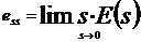
一、實驗目的: 1、觀測0型系統的脈沖響應、階躍響應和斜坡響應,并測量穩態誤差; 2、觀測Ⅰ型系統的脈沖響應、階躍響應和斜坡響應,并測量穩態誤差; 3、觀測Ⅱ型系統的脈沖響應、斜坡響應和拋物線響應,并測量穩態誤差。 二、實驗內容: 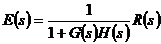
設系統開環傳遞函數一般表達式為 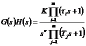 (n≥m) (n≥m)
則系統的穩態誤差可表示為 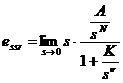
設 0型系統的開環傳遞函數為 Ⅰ型系統的開環傳遞函數為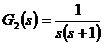 Ⅱ型系統的開環傳遞函數為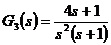 實驗問題:6、系統開環傳遞函數如下 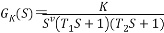
T1=0.3,T2=0.4,要求如下: - v=0;K=1,3,5,8時觀察系統階躍響應和斜坡響應,并測量其穩態誤差;
- v=1; K=1,3,5,8時觀察系統階躍響應和斜坡響應,并測量其穩態誤差;
- v=2; K=1,3,5,8時觀察系統階躍響應和斜坡響應,并測量其穩態誤差;
- 說明系統型別和K的參數對穩態誤差的影響。
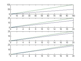
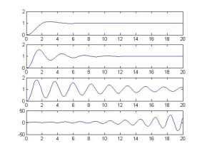
- (1)v=0;K=1,3,5,8時觀察系統階躍響應和斜坡響應,并測量其穩態誤差
階躍程序:t=0:0.1:20
[num1,den1]=cloop([1],[0.12 0.7 1]);
[num2,den2]=cloop([3],[0.12 0.7 1]);
[num3,den3]=cloop([5],[0.12 0.7 1]);
[num4,den4]=cloop([8],[0.12 0.7 1]);
y1=step(num1,den1,t);
y2=step(num2,den2,t);
y3=step(num3,den3,t);
y4=step(num4,den4,t);
subplot(411);plot(t,y1);
subplot(412);plot(t,y2);
subplot(413);plot(t,y3);
subplot(414);plot(t,y4);
er1=1-y1(length(t));
er2=1-y2(length(t));
er3=1-y3(length(t));
er4=1-y4(length(t));
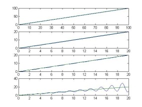
斜坡程序:t=0:0.1:20
t1=0:0.1:100;
[num1,den1]=cloop([1],[0.12 0.7 1]);
[num2,den2]=cloop([3],[0.12 0.7 1]);
[num3,den3]=cloop([5],[0.12 0.7 1]);
[num4,den4]=cloop([8],[0.12 0.7 1]);
y1=step(num1,[den1 0],t1);
y2=step(num2,[den2 0],t);
y3=step(num3,[den3 0],t);
y4=step(num4,[den4 0],t);
subplot(411);plot(t1,y1,t1,t1);
subplot(412);plot(t,y2,t,t);
subplot(413);plot(t,y3,t,t);
subplot(414);plot(t,y4,t,t);
er1=t1(length(t1))-y1(length(t1));
er2=t(length(t))-y2(length(t));
er3=t(length(t))-y3(length(t));
er4=t(length(t))-y4(length(t));

(2)v=1;K=1,3,5,8時觀察系統階躍響應和斜坡響應,并測量其穩態誤差
階躍程序:t=0:0.1:20
[num1,den1]=cloop([1],[0.12 0.7 1 0]);
[num2,den2]=cloop([3],[0.12 0.7 1 0]);
[num3,den3]=cloop([5],[0.12 0.7 1 0]);
[num4,den4]=cloop([8],[0.12 0.7 1 0]);
y1=step(num1,den1,t);
y2=step(num2,den2,t);
y3=step(num3,den3,t);
y4=step(num4,den4,t);
subplot(411);plot(t,y1);
subplot(412);plot(t,y2);
subplot(413);plot(t,y3);
subplot(414);plot(t,y4);
er1=1-y1(length(t));
er2=1-y2(length(t));
er3=1-y3(length(t));
er4=1-y4(length(t));
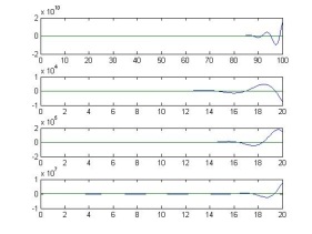
斜坡程序:t=0:0.1:20
t1=0:0.1:100;
[num1,den1]=cloop([1],[0.12 0.7 1 0]);
[num2,den2]=cloop([3],[0.12 0.7 1 0]);
[num3,den3]=cloop([5],[0.12 0.7 1 0]);
[num4,den4]=cloop([8],[0.12 0.7 1 0]);
y1=step(num1,[den1 0],t1);
y2=step(num2,[den2 0],t);
y3=step(num3,[den3 0],t);
y4=step(num4,[den4 0],t);
subplot(411);plot(t1,y1,t1,t1);
subplot(412);plot(t,y2,t,t);
subplot(413);plot(t,y3,t,t);
subplot(414);plot(t,y4,t,t);
er1=t1(length(t1))-y1(length(t1));
er2=t(length(t))-y2(length(t));
er3=t(length(t))-y3(length(t));
er4=t(length(t))-y4(length(t));
- (3)v=2;K=1,3,5,8時觀察系統階躍響應和斜坡響應,并測量其穩態誤差;
階躍程序:t=0:0.1:20 [num1,den1]=cloop([1],[0.12 0.7 1 0 0]); [num2,den2]=cloop([3],[0.12 0.7 1 0 0]); [num3,den3]=cloop([5],[0.12 0.7 1 0 0]); [num4,den4]=cloop([8],[0.12 0.7 1 0 0]); y1=step(num1,den1,t); y2=step(num2,den2,t); y3=step(num3,den3,t); y4=step(num4,den4,t); subplot(411);plot(t,y1); subplot(412);plot(t,y2); subplot(413);plot(t,y3); subplot(414);plot(t,y4); er1=1-y1(length(t)); er2=1-y2(length(t)); er3=1-y3(length(t)); er4=1-y4(length(t)); 斜坡程序:t=0:0.1:20 t1=0:0.1:100; [num1,den1]=cloop([1],[0.12 0.7 1 0]); [num2,den2]=cloop([3],[0.12 0.7 1 0]); [num3,den3]=cloop([5],[0.12 0.7 1 0]); [num4,den4]=cloop([8],[0.12 0.7 1 0]); y1=step(num1,[den1 0],t1); y2=step(num2,[den2 0],t); y3=step(num3,[den3 0],t); y4=step(num4,[den4 0],t); subplot(411);plot(t1,y1,t1,t1); subplot(412);plot(t,y2,t,t); subplot(413);plot(t,y3,t,t); subplot(414);plot(t,y4,t,t); er1=t1(length(t1))-y1(length(t1)); er2=t(length(t))-y2(length(t)); er3=t(length(t))-y3(length(t)); er4=t(length(t))-y4(length(t)); 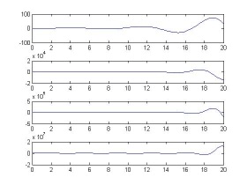
(4)說明系統型別和K的參數對穩態誤差的影響。 在階躍輸入作用下,僅0型系統有穩態誤差,其大小與階躍輸入的幅值成正比,與系統的開環增益成反比。對I型及I型以上的系統,其穩態誤差為0 在斜坡輸入之下,0型系統的輸出量不能跟蹤其輸入量的變化,這是因為輸出量的速度小于輸入量的速度,導致兩者的差距不斷增大,穩態誤差趨于無窮大,穩態時,I型系統的輸出量與輸入量雖以相同的速度變化,但前者較后者在位置上落后一個常量,這個常量就是穩態誤差。穩態情況下II型及II型以系統的輸出量與輸入量不僅速度相等,而且位置相同。
完整的Word格式文檔51黑下載地址:
 實驗四實驗報告.docx
(161.5 KB, 下載次數: 6)
實驗四實驗報告.docx
(161.5 KB, 下載次數: 6)
2019-6-10 18:55 上傳
點擊文件名下載附件
穩態誤差分析 下載積分: 黑幣 -5
|


 QQ好友和群
 QQ空間
QQ空間 騰訊微博
騰訊微博 騰訊朋友
騰訊朋友 收藏
收藏 淘帖
淘帖 頂
頂 踩
踩